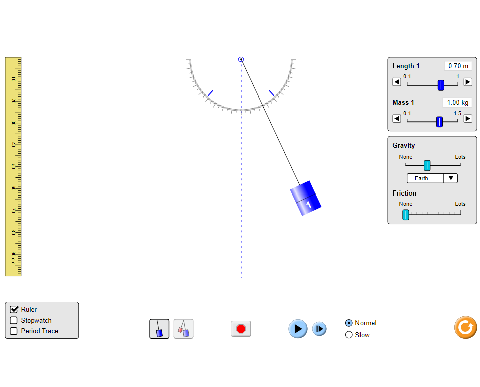
The following lab can be replicated in person by using an eraser as the pendulum bob, string, a ruler and a stopwatch.
Theory
The period of a simple pendulum is given by the formula: $$T=2\pi\sqrt{\frac{l}{g}}$$
If we square both sides of this equation, we get the following: $$\color{limegreen}T^2\color{black}=\color{slateblue}\frac{4\pi^2}{g}\color{red}l\color{black}+0$$
If we compare this to the standard form of the equation of a straight line: $$\color{limegreen}y\color{black}=\color{slateblue}m\color{red}x\color{black}+c$$
We see that by plotting the period squared ($T^2$) versus the length ($l$), the y-intercept of the best-fit line will be zero(0) and the gradient will be: $$m=\frac{4\pi^2}{g}$$
We can thus find an approximation for acceleration due to gravity($g$) using the gradient of the best-fit line: $$g=\frac{4\pi^2}{m}$$
Aim
To determine the relationship between the length and period of a simple pendulum
Materials/Apparatus
Diagram

Method
- Run the simulation
- Select ‘Intro’
- Enable the ‘Stopwatch’ option
- Set the length of the pendulum to 50 cm (0.5 m)
- Pause the simulation
- Drag the pendulum to an angle of 30 degrees
- Start the stopwatch
- Play the simulation then pause it after the pendulum completes 10 oscillations
- Record the time seen on the stopwatch
- Reset the stopwatch
- Repeat steps 5 to 10 for the same length of 50 cm two more times
- Repeat this process for the other lengths stated in the table below
Results
| Length/$m$ | Time for 10 oscillations/$s$ | Time for 1 oscillation/$s$ |
|---|---|---|
| 0.10 | ||
| 0.15 | ||
| 0.20 | ||
| 0.25 | ||
| 0.30 | ||
| 0.35 | ||
| 0.40 | ||
| 0.45 | ||
| 0.50 |
Data Analysis
- Plot a graph of the square of the period of the pendulum (in $s^2$) versus its length (in $m$)
- Draw a best fit line to represent the data
- Find the gradient of the best fit line
- Use the simple pendulum formula to find the value of acceleration due to gravity ($g$)
